31. Markov Assumption for Observation Model

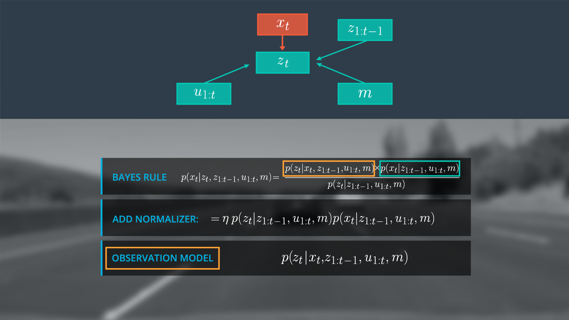
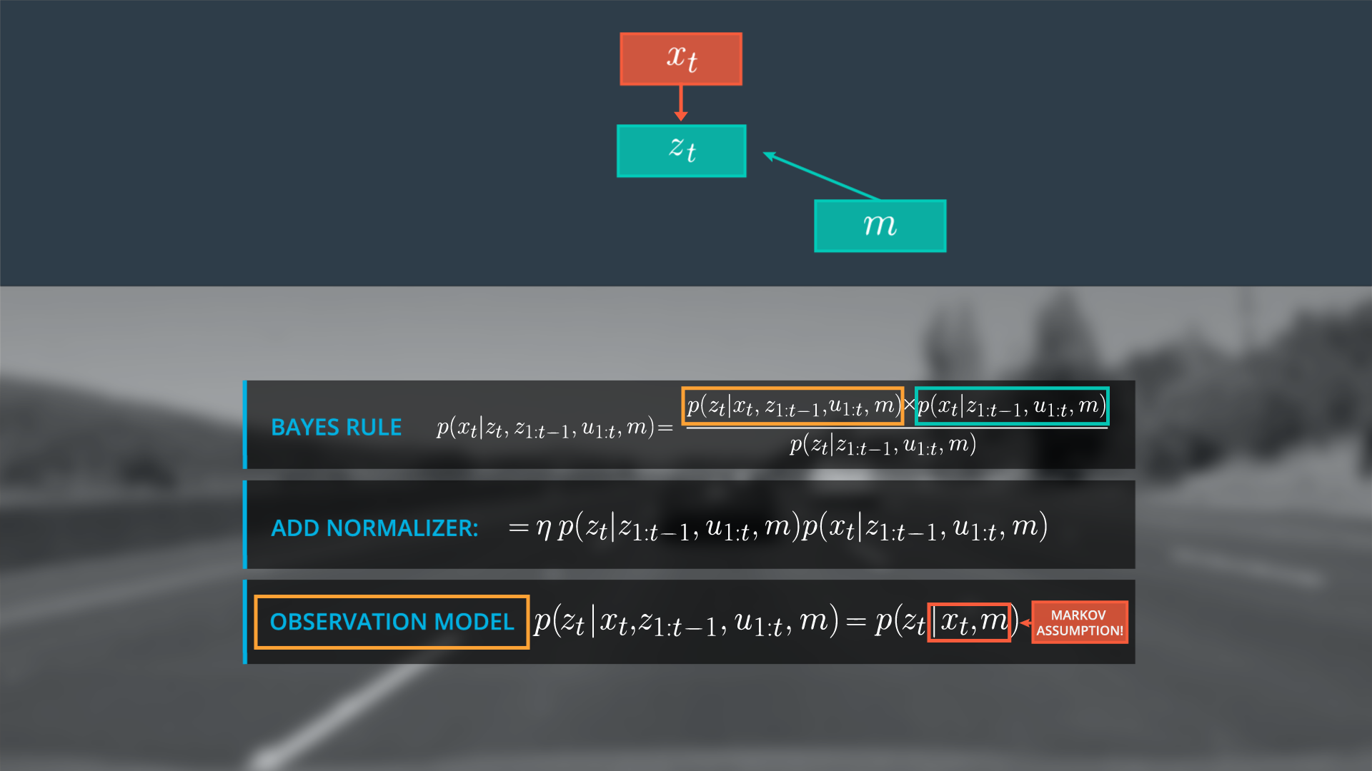
The Markov assumption can help us simplify the observation model. Recall that the Markov Assumption is that the next state is dependent only upon the preceding states and that preceding state information has already been used in our state estimation. As such, we can ignore terms in our observation model prior to x_t since these values have already been accounted for in our current state and assume that t is independent of previous observations and controls.

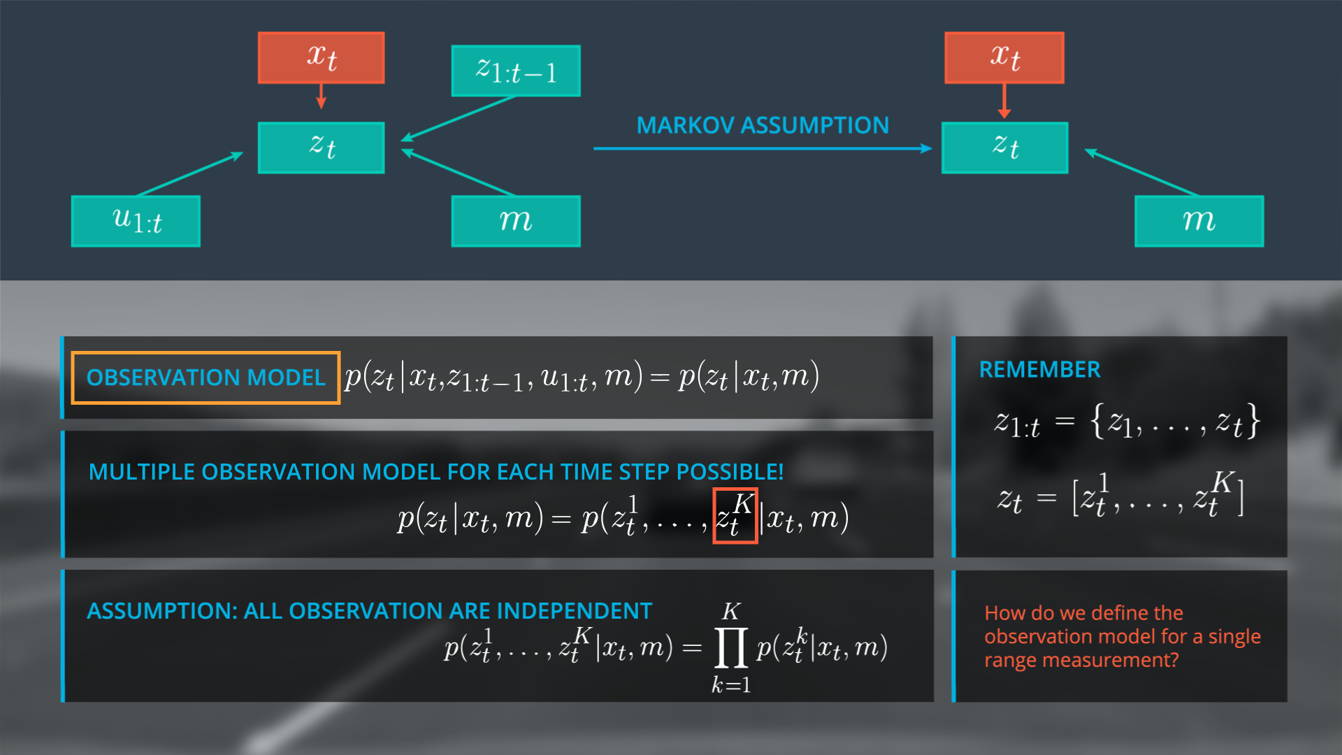
With these assumptions we simplify our posterior distribution such that the observations at t are dependent only on x at time t and the map.

Since z_t can be a vector of multiple observations we rewrite our observation model to account for the observation models for each single range measurement. We assume that the noise behavior of the individual range values z_t^1 to z_t^k is independent and that our observations are independent, allowing us to represent the observation model as a product over the individual probability distributions of each single range measurement. Now we must determine how to define the observation model for a single range measurement.

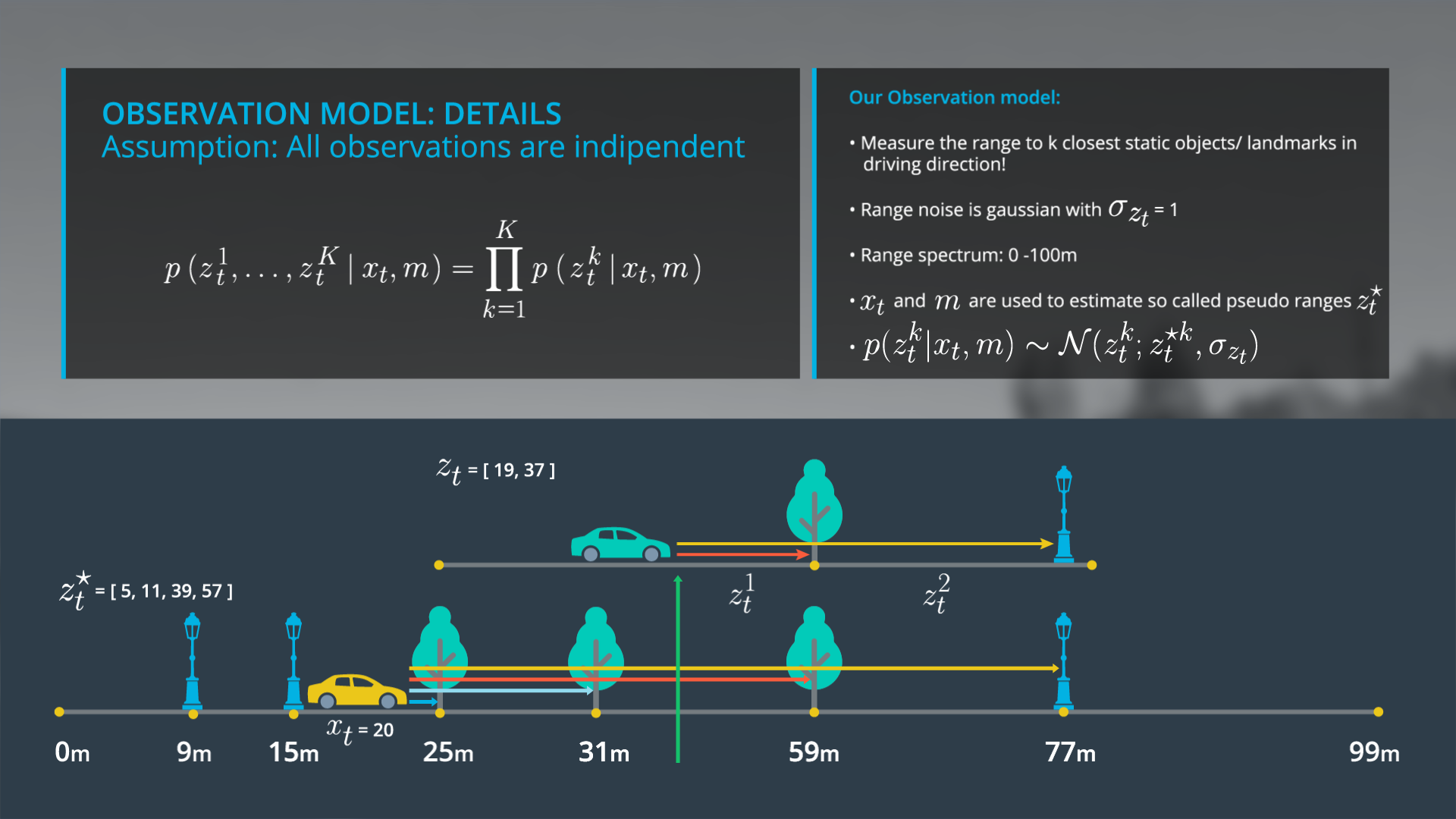
In general there exists a variety of observation models due to different sensor, sensor specific noise behavior and performance, and map types. For our 1D example we assume that our sensor measures to the n closest objects in the driving direction, which represent the landmarks on our map. We also assume that observation noise can be modeled as a Gaussian with a standard deviation of 1 meter and that our sensor can measure in a range of 0 – 100 meters.

To implement the observation model we use the given state x_t , and the given map to estimate pseudo ranges, which represent the true range values under the assumption that your car would stand at a specific position x_t , on the map. For example, if our car is standing at position 20 it would make use x_t , and m to make pseudo range ( z_t^* ) observations in the order of the first landmark to the last landmark or 5, 11, 39, and 57 meters. Compared to our real observations ( z_t = [19, 37]) the position x_t , = 20 seems unlikely and our observation would rather fit to a position around 40.

Based on this example the observation model for a single range measurement is defined by the probability of the following normal distribution p(z_t^k|x_t )\tilde\ N(z_t^k,z_t^{ k},\sigma z_t) where z_t^{ k} is the mean. This insight will ultimately allow us to implement the observation model in c++.